Pipelines

Pipelines allow users to compose filters that transform the published input data into new meshes. This is where users specify typical geometric transforms (e.g., clipping and slicing), field based transforms (e.g., threshold and contour), etc. The resulting data from each Pipeline can be used as input to Scenes or Extracts. Each pipeline contains one or more filters that transform the published mesh data. When more than one filter is specified, each successive filter consumes the result of the previous filter, and filters are executed in the order in which they are declared.

The code below shows how to declare two pipelines, and generate images of the pipeline results. The first applies a contour filter to extract two isosurfaces of the scalar field noise. The second pipeline applies a threshold filter to screen the noise field, and then a clip filter to extract the intersection of what remains from the threshold with a sphere.

conduit::Node pipelines;
// pipeline 1
pipelines["pl1/f1/type"] = "contour";
// filter parameters
conduit::Node contour_params;
contour_params["field"] = "noise";
constexpr int num_iso_values = 2;
double iso_values[num_iso_values] = {0.0, 0.5};
contour_params["iso_values"].set_external(iso_values, num_iso_values);
pipelines["pl1/f1/params"] = contour_params;

// pipeline 2
pipelines["pl2/f1/type"] = "threshold";
// filter parameters
conduit::Node thresh_params;
thresh_params["field"]  = "noise";
thresh_params["min_value"] = 0.0;
thresh_params["max_value"] = 0.5;
pipelines["pl2/f1/params"] = thresh_params;

pipelines["pl2/f2/type"]   = "clip";
// filter parameters
conduit::Node clip_params;
clip_params["topology"] = "mesh";
clip_params["sphere/center/x"] = 0.0;
clip_params["sphere/center/y"] = 0.0;
clip_params["sphere/center/z"] = 0.0;
clip_params["sphere/radius"]   = .1;
pipelines["pl2/f2/params/"] = clip_params;

// make some imaages of the data
conduit::Node scenes;
// add a plot of pipeline 1
scenes["s1/plots/p1/type"] = "pseudocolor";
scenes["s1/plots/p1/pipeline"] = "pl1";
scenes["s1/plots/p1/field"] = "noise";

// add a plot of pipeline 2
scenes["s2/plots/p1/type"] = "pseudocolor";
scenes["s2/plots/p1/pipeline"] = "pl2";
scenes["s2/plots/p1/field"] = "noise";

// setup actions
conduit::Node actions;

conduit::Node add_pipelines = actions.append();
add_pipelines["action"] = "add_pipelines";
add_pipelines["pipelines"] = pipelines;

conduit::Node add_scenes = actions.append();
add_scenes["action"] = "add_scenes";
add_scenes["scenes"] = scenes;

actions.append()["action"] = "execute";

Ascent ascent;
ascent.open();
ascent.publish(mesh); // mesh not shown
ascent.execute(actions);
ascent.close();

Ascent and VTK-h are under heavy development and features are being added rapidly. As we stand up the infrastructure necessary to support a wide variety filter we created the following filters for the alpha release:

• Contour

• Threshold

• Slice

• Three Slice

• Automatic Slice

• Clip

• Clip by field

• Isovolume

• Vector magnitude

In the following section we provide brief descriptions and code examples of the supported filters. For complete code examples, please consult the unit tests located in src/tests/ascent..

Filters

Our filter API consists of the type of filter and the parameters associated with the filter in the general form:

{
  "type"   : "filter_name",
  "params":
  {
    "string_param" : "string",
    "double_param" : 2.0
  }
}

In c++, the equivalent declarations would be as follows:

conduit::Node filter;
filter["type"] = "filter_name";
filter["params/string_param"] = "string";
filter["params/double_param"] = 2.0;

Included Filters

Contour

The contour filter evaluates a node-centered scalar field for all points at a given iso-value. This results in a surface if the iso-value is within the scalar field. iso_vals can contain a single double or an array of doubles. Additionally, instead of specifying exact iso-values, a number of ‘levels’ can be entered. In this case, iso-values will be created evenly spaced through the scalar range. For example, if the scalar range is [0.0, 1.0] and ‘levels’ is set to 3, then the iso-values (0.25, 0.5, 0.75) will be created. The code below provides examples creating a pipeline using all three methods:

conduit::Node pipelines;
// pipeline 1
pipelines["pl1/f1/type"] = "contour";
// filter knobs
conduit::Node &contour_params = pipelines["pl1/f1/params"];
contour_params["field"] = "braid";
contour_params["iso_values"] = -0.4;

conduit::Node pipelines;
// pipeline 1
pipelines["pl1/f1/type"] = "contour";
// filter knobs
conduit::Node &contour_params = pipelines["pl1/f1/params"];
contour_params["field"] = "braid";
constexpr int num_iso_values = 3;
double iso_vals[num_iso_values] = {-0.4, 0.2, 0.4};
contour_params["iso_values"].set_external(iso_vals, num_iso_values);

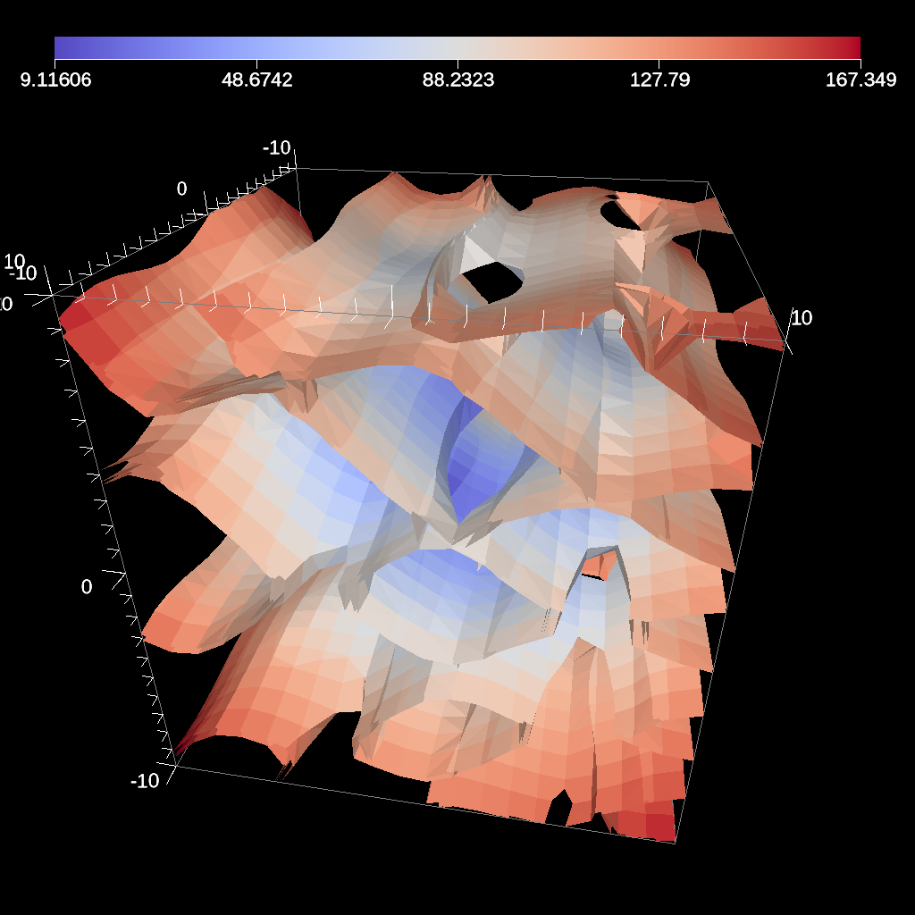
Fig. 25 An example image of multiple contours produced using the previous code sample.

conduit::Node pipelines;
// pipeline 1
pipelines["pl1/f1/type"] = "contour";
// filter knobs
conduit::Node &contour_params = pipelines["pl1/f1/params"];
contour_params["field"] = "braid";
contour_params["levels"] = 5;

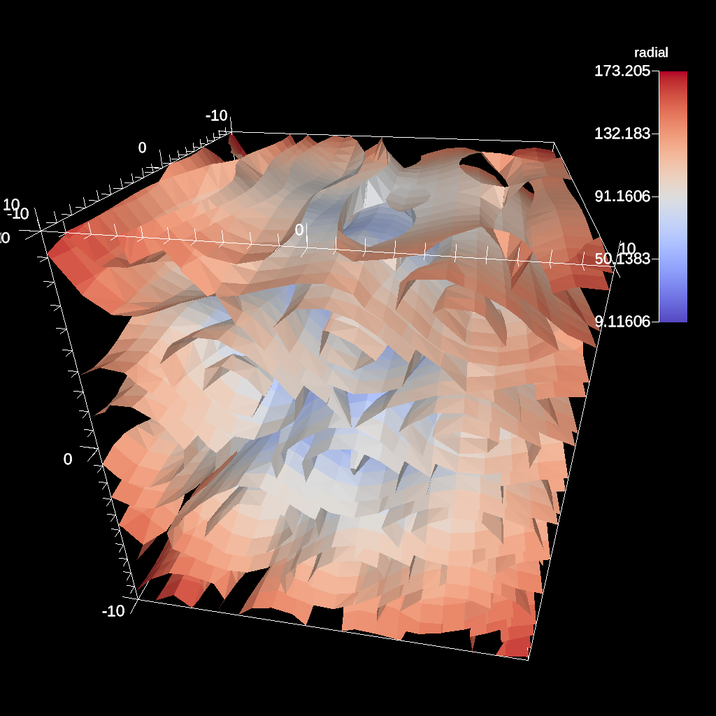
Fig. 26 An example of creating five evenly spaced iso-values through a scalar field.

Figure 25 shows an image produced from multiple contours. All contour examples are located in the test in the file contour test.

Threshold

The threshold filter removes cells that are not contained within a specified scalar range.

conduit::Node pipelines;
// pipeline 1
pipelines["pl1/f1/type"] = "threshold";
// filter knobs
conduit::Node &thresh_params = pipelines["pl1/f1/params"];
thresh_params["field"] = "braid";
thresh_params["min_value"] = -0.2;
thresh_params["max_value"] = 0.2;

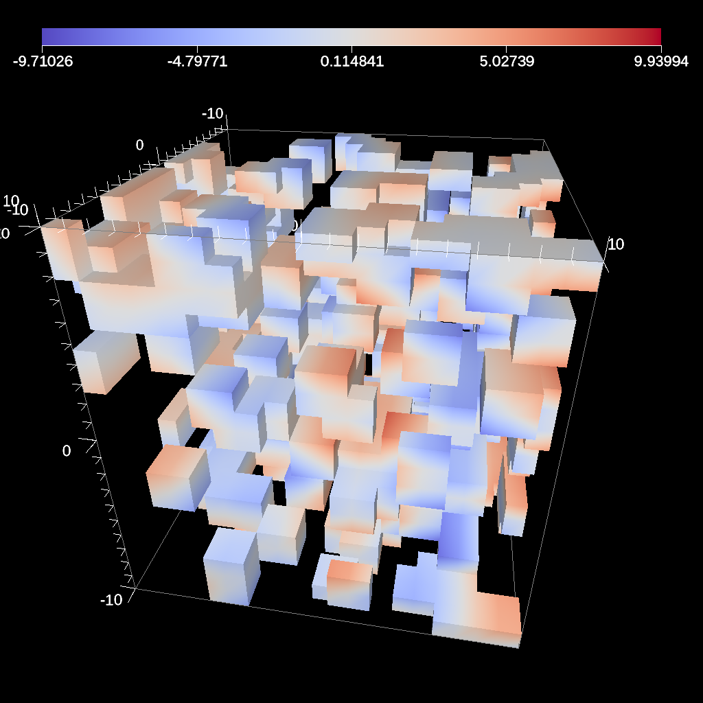
Fig. 27 An example image of the threshold filter using the previous code sample.

Figure 27 shows an image produced from a threshold filter. The full example is located in the file threshold test.

Slice

The slice filter extracts a 2d plane from a 3d data set. The plane is defined by a point (on the plane) and a normal vector (not required to be normalized).

conduit::Node pipelines;
pipelines["pl1/f1/type"] = "slice";
// filter knobs
conduit::Node &slice_params = pipelines["pl1/f1/params"];
slice_params["point/x"] = 0.f;
slice_params["point/y"] = 0.f;
slice_params["point/z"] = 0.f;

slice_params["normal/x"] = 0.f;
slice_params["normal/y"] = 0.f;
slice_params["normal/z"] = 1.f;

Fig. 28 An example image of the slice filter on a element-centered variable using the previous code sample.

Figure 28 shows an image produced from the slice filter. The full example is located in the file slice test.

Three Slice

The three slice filter slices 3d data sets using three axis-aligned slice planes and leaves the resulting planes in 3d where they can all be viewed at the same time. Three slice is meant primarily for quick visual exploration of 3D data where the internal features cannot be readily observed from the outside.

The slice planes will automatically placed at the center of the data sets spatial extents. Optionally, offsets for each plane can be specified. Offsets for each axis are specified by a floating point value in the range [-1.0, 1.0], where -1.0 places the plane at the minimum spatial extent on the axis, 1.0 places the plane at the maximum spatial extent on the axis, and 0.0 places the plane at the center of the spatial extent. By default, all three offsets are 0.0.

conduit::Node pipelines;
pipelines["pl1/f1/type"] = "3slice";

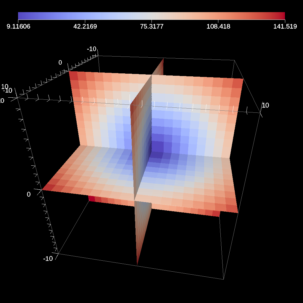
Fig. 29 An example image of the three slice filter on a element-centered variable using the previous code sample with automatic slice plane placement.

conduit::Node pipelines;
pipelines["pl1/f1/type"] = "3slice";

// filter knobs (all these are optional)
conduit::Node &slice_params = pipelines["pl1/f1/params"];
slice_params["x_offset"] = 1.f;   // largest value on the x-axis
slice_params["y_offset"] = 0.f;   // middle of the y-axis
slice_params["z_offset"] = -1.f;  // smalles value of the z-axis

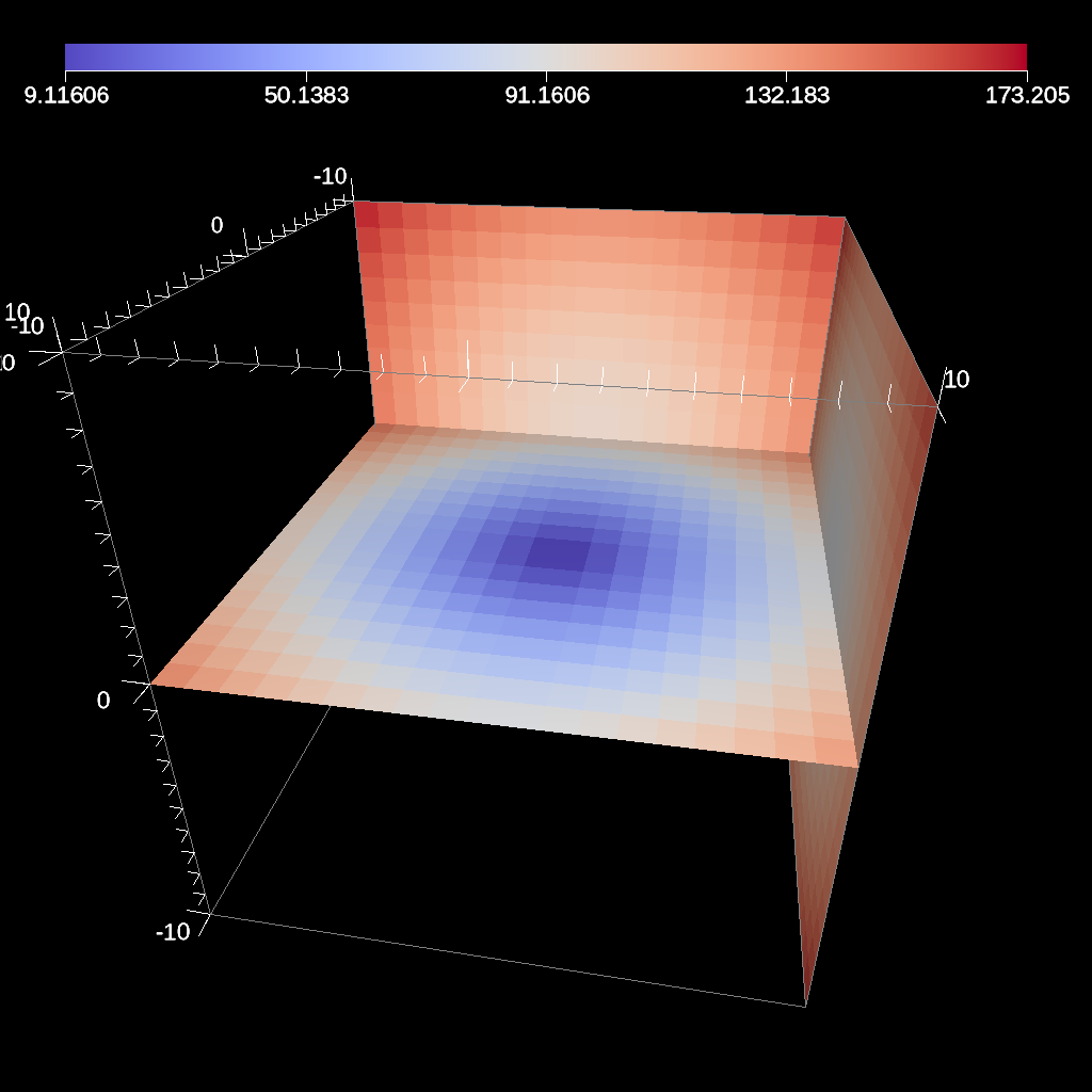
Fig. 30 An example image of the three slice filter on a element-centered variable using the previous code sample with user specified offsets for each axis.

Figures 29 and 30 show an images produced from the three slice filter. The full example is located in the file slice test.

Automatic Slice

The automatic slice filter extracts a 2d plane from a 3d data set by slicing the data set in a user-specified direction a user-specified number of times, and then selects the slice that has the highest entropy for the user-specified field. The slicing direction of the data set is determined by a normal (not required to be normalized), and the number of slices evaluated is specified by the number of levels, which will equally space the slices in the normal direction. Automatic slice is meant primarily for quick visual exploration of 3D data where the internal features cannot be readily observed from the outside.

The slice planes will be automatically placed based on the normal provided and the number of levels specified. The final output slice will be the slice that has the highest entropy for the specified field.

Depending on the normal provided, the rendering camera may need to be adjusted in order to view the chosen slice. By default, the camera is pointed down the z-axis, so a normal of (0,0,1) does not need any adjusting. In contrast, if the normal is (1,0,0), the camera needs to be adjusted to point down the x-axis, this can be done by adjusting the azimuth to rotate the camera horizontally around data set. Additionally, if the normal is (0,1,0) and the camera needs to point down the y-axis, this can be achieved by using the elevation camera parameter to rotate the camera vertically around the data set.

conduit::Node pipelines;
pipelines["pl1/f1/type"] = "auto_slice";

// filter knobs (not optional)
conduit::Node &slice_params = pipelines["pl1/f1/params"];
slice_params["normal/x"] = 0.f;
slice_params["normal/y"] = 0.f;
slice_params["normal/z"] = 1.f;
slice_params["field"] = "braid";
slice_params["levels"] = 10;

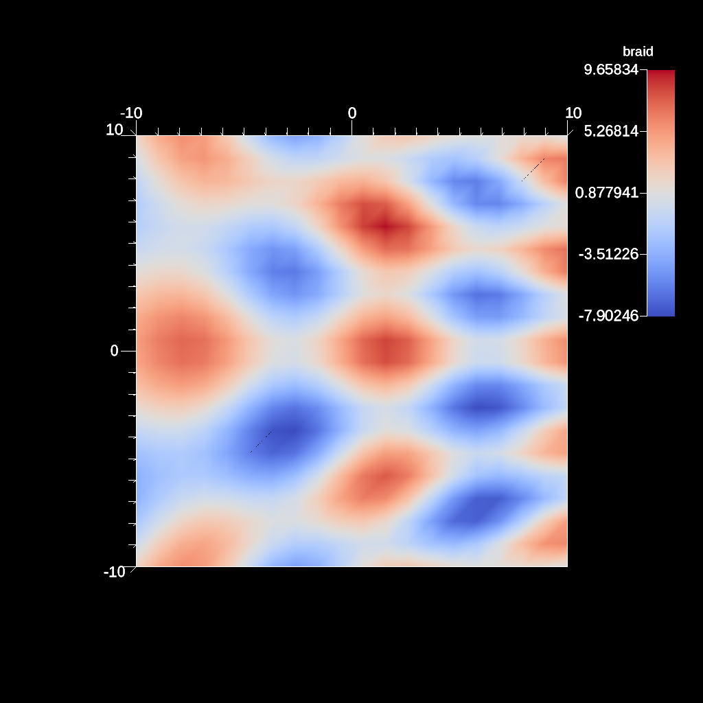
Fig. 31 An example image of the automatic slice filter using the previous code sample. This example uses a normal that points down the z-axis, the same as the default camera.

conduit::Node pipelines;
pipelines["pl1/f1/type"] = "auto_slice";

// filter knobs (not optional)
conduit::Node &slice_params = pipelines["pl1/f1/params"];
slice_params["normal/x"] = 1.f;
slice_params["normal/y"] = 0.f;
slice_params["normal/z"] = 0.f;
slice_params["field"] = "braid";
slice_params["levels"] = 10;

conduit::Node scenes;
// add a plot of pipeline 1
scenes["s1/plots/p1/type"] = "pseudocolor";
scenes["s1/plots/p1/pipeline"] = "pl1";
scenes["s1/plots/p1/field"] = "braid";
//Need to turn camera 90 degrees horizontally
//in order to point down x-axis
scenes["s1/renders/r1/camera/azimuth"] = 90.0;
scenes["s1/renders/r1/image_prefix"]     = output_file;

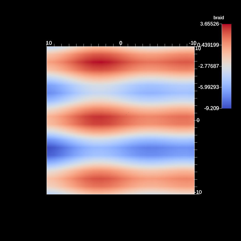
Fig. 32 An example image of the automatic slice filter using the previous code sample. This example uses a normal that points down the x-axis, meaning the angle camera needs to be adjusted using the azimuth.

conduit::Node pipelines;
pipelines["pl1/f1/type"] = "auto_slice";

// filter knobs (not optional)
conduit::Node &slice_params = pipelines["pl1/f1/params"];
slice_params["normal/x"] = 0.f;
slice_params["normal/y"] = 1.f;
slice_params["normal/z"] = 0.f;
slice_params["field"] = "braid";
slice_params["levels"] = 10;

conduit::Node scenes;
// add a plot of pipeline 1
scenes["s1/plots/p1/type"] = "pseudocolor";
scenes["s1/plots/p1/pipeline"] = "pl1";
scenes["s1/plots/p1/field"] = "braid";
//Need to turn camera 90 degrees vertically
//in order to point down y-axis
scenes["s1/renders/r1/camera/elevation"] = 90.0;
scenes["s1/renders/r1/image_prefix"]     = output_file;

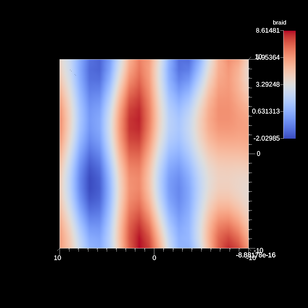
Fig. 33 An example image of the automatic slice filter using the previous code sample. This example uses a normal that points down the y-axis, meaning the angle camera needs to be adjusted using the elevation.

conduit::Node pipelines;
pipelines["pl1/f1/type"] = "auto_slice";

// filter knobs (not optional)
conduit::Node &slice_params = pipelines["pl1/f1/params"];
slice_params["normal/x"] = 1.f;
slice_params["normal/y"] = 1.f;
slice_params["normal/z"] = 0.f;
slice_params["field"] = "braid";
slice_params["levels"] = 10;

conduit::Node scenes;
// add a plot of pipeline 1
scenes["s1/plots/p1/type"] = "pseudocolor";
scenes["s1/plots/p1/pipeline"] = "pl1";
scenes["s1/plots/p1/field"] = "braid";
//Need to turn camera
//90 degrees horizontally
//and 45 degrees vertically
//based on normal
scenes["s1/renders/r1/camera/azimuth"] = 90.0;
scenes["s1/renders/r1/camera/elevation"] = 45.0;
scenes["s1/renders/r1/image_prefix"]     = output_file;

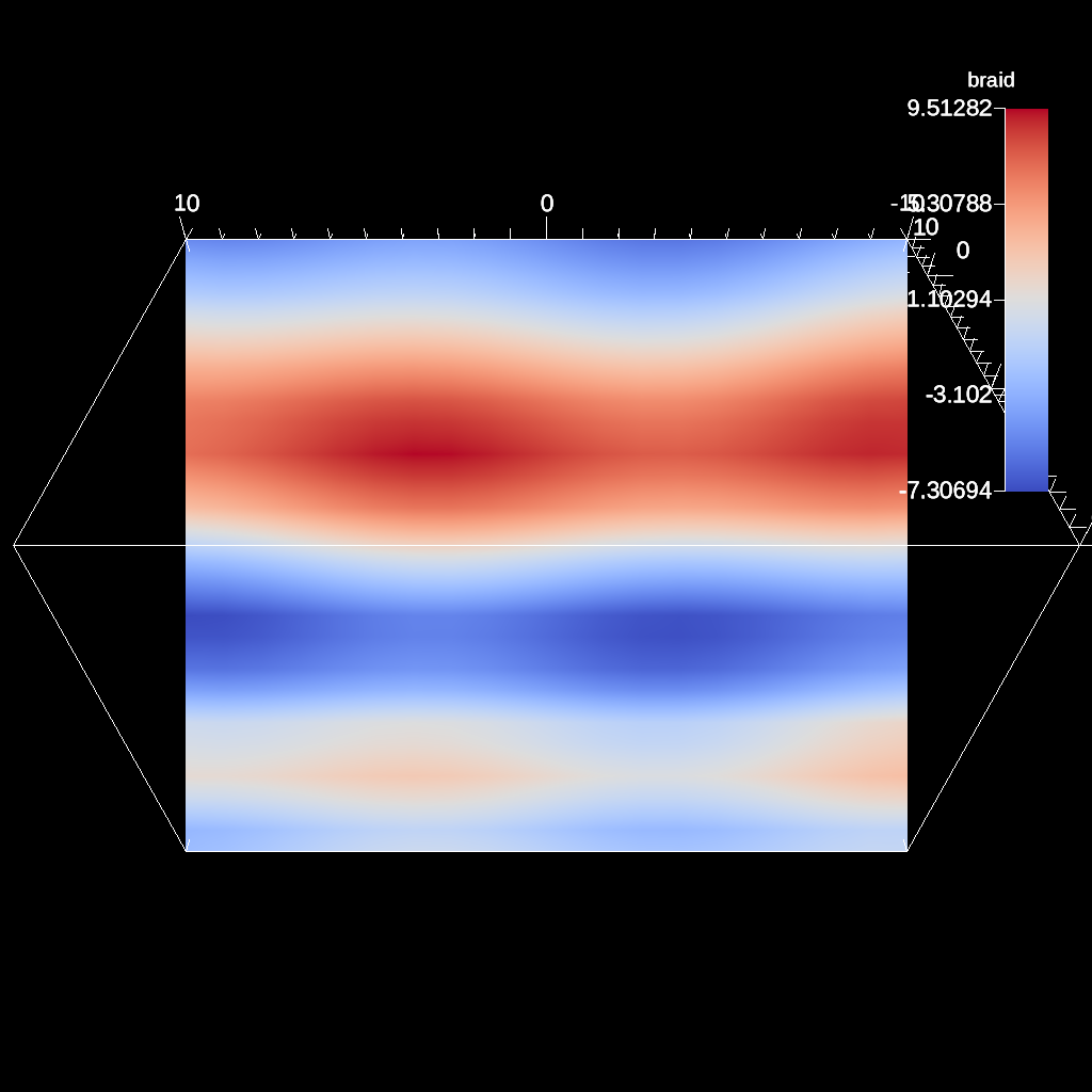
Fig. 34 An example image of the automatic slice filter using the previous code sample. This example uses a normal that points in the xy-direction, meaning the angle camera needs to be adjusted using both the azimuth and elevation.

Figures 31, 32 , 33 , and 34 show images produced from the automatic slice filter. The full example is located in the file slice test.

Clip

The clip filter removes cells from the specified topology using implicit functions. By default, only the area outside of the implicit function remains, but the clip can be inverted. There are three implicit functions that clip can use: sphere, box, and plane.

// define a clip by a sphere
conduit::Node pipelines;
// pipeline 1
pipelines["pl1/f1/type"] = "clip";
// filter knobs
conduit::Node &clip_params = pipelines["pl1/f1/params"];
clip_params["topology"] = "mesh";
clip_params["sphere/radius"] = 11.;
clip_params["sphere/center/x"] = 0.;
clip_params["sphere/center/y"] = 0.;
clip_params["sphere/center/z"] = 0.;

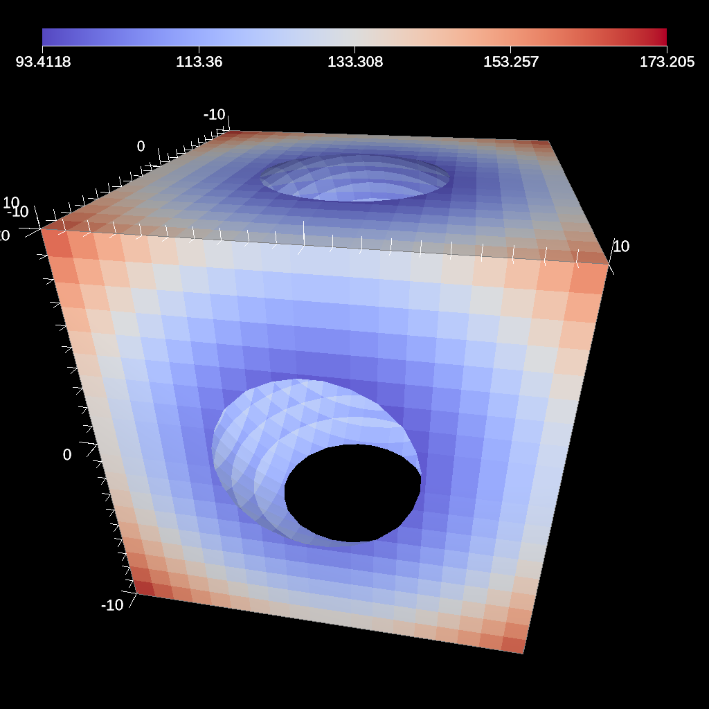
Fig. 35 An example image of the clip filter using the previous code sample. The data set is a cube with extents from (-10, -10, -10) to (10, 10, 10), and the code removes a sphere centered at the origin with a radius of 11.

conduit::Node pipelines;
// pipeline 1
pipelines["pl1/f1/type"] = "clip";
// filter knobs
conduit::Node &clip_params = pipelines["pl1/f1/params"];
clip_params["topology"] = "mesh";
clip_params["invert"] = "true";
clip_params["sphere/radius"] = 11.;
clip_params["sphere/center/x"] = 0.;
clip_params["sphere/center/y"] = 0.;
clip_params["sphere/center/z"] = 0.;

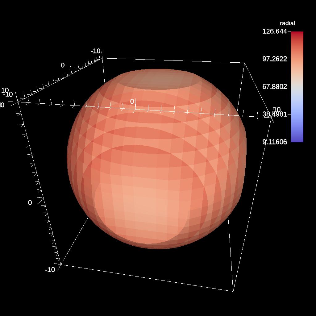
Fig. 36 An example of the same sphere clip, but in this case, the clip is inverted.

// define a clip by a box
conduit::Node pipelines;
// pipeline 1
pipelines["pl1/f1/type"] = "clip";
// filter knobs
conduit::Node &clip_params = pipelines["pl1/f1/params"];
clip_params["topology"] = "mesh";
clip_params["box/min/x"] = 0.;
clip_params["box/min/y"] = 0.;
clip_params["box/min/z"] = 0.;
clip_params["box/max/x"] = 10.01; // <=
clip_params["box/max/y"] = 10.01;
clip_params["box/max/z"] = 10.01;

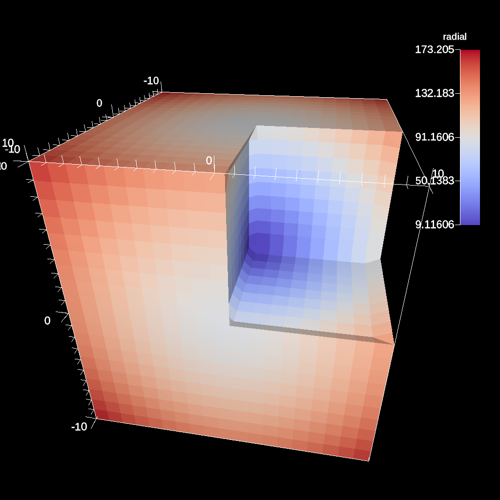
Fig. 37 A box clip of the same data set that removes the octant on the positive x, y, and z axes.

conduit::Node pipelines;
// pipeline 1
pipelines["pl1/f1/type"] = "clip";
// filter knobs
conduit::Node &clip_params = pipelines["pl1/f1/params"];
clip_params["topology"] = "mesh";
clip_params["plane/point/x"] = 0.;
clip_params["plane/point/y"] = 0.;
clip_params["plane/point/z"] = 0.;
clip_params["plane/normal/x"] = 1.;
clip_params["plane/normal/y"] = 0.;
clip_params["plane/normal/z"] = 0;

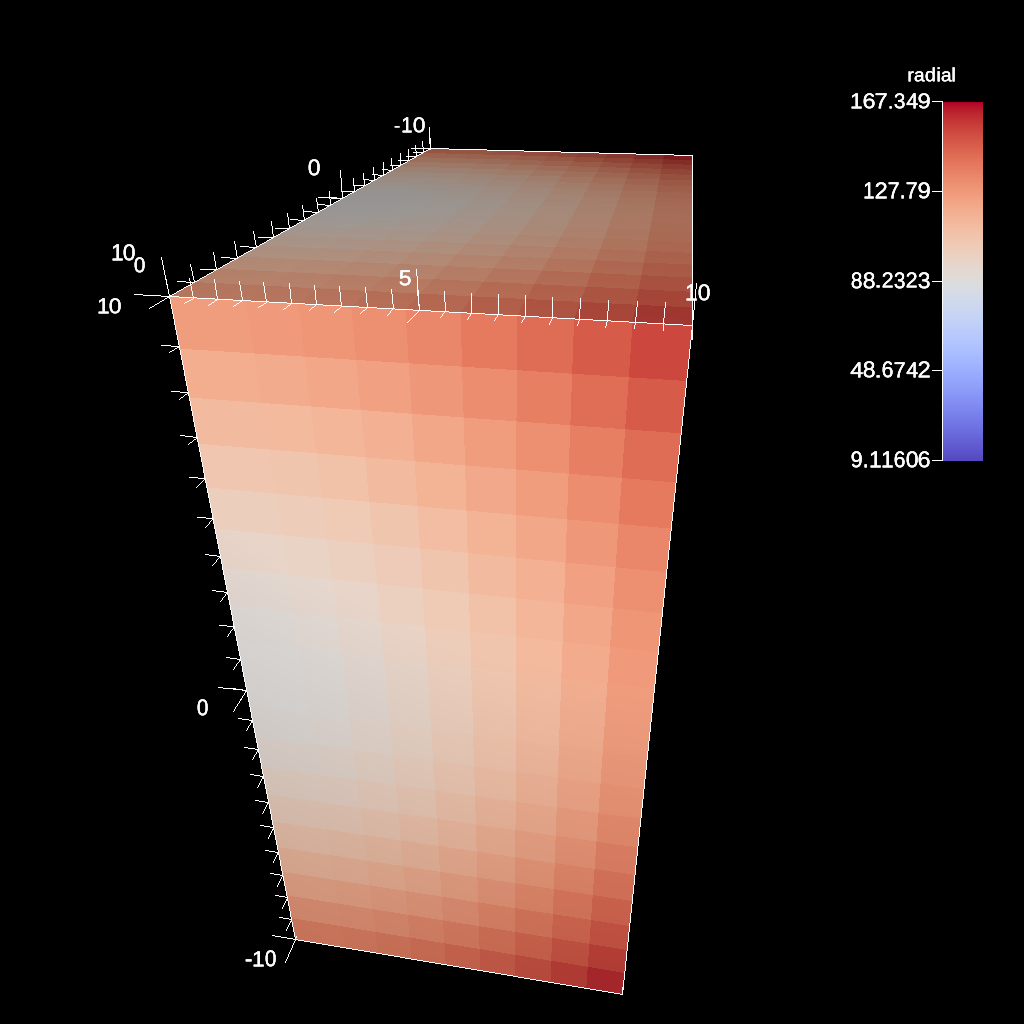
Fig. 38 Clipping by a plane defined by a point on the plane and the plane normal.

Figures 35, 36, 37, and 38 show an images produced from the clip filter. All of the clip examples are located in the file clip test.

Clip By Field

The clip by field filter removes cells from the specified topology using the values in a scalar field. By default, all values below the clip value are removed from the data set. As with clip by implicit function, the clip can be inverted.

conduit::Node pipelines;
// pipeline 1
pipelines["pl1/f1/type"] = "clip_with_field";
// filter knobs
conduit::Node &clip_params = pipelines["pl1/f1/params"];
clip_params["field"] = "braid";
clip_params["clip_value"] = 0.;

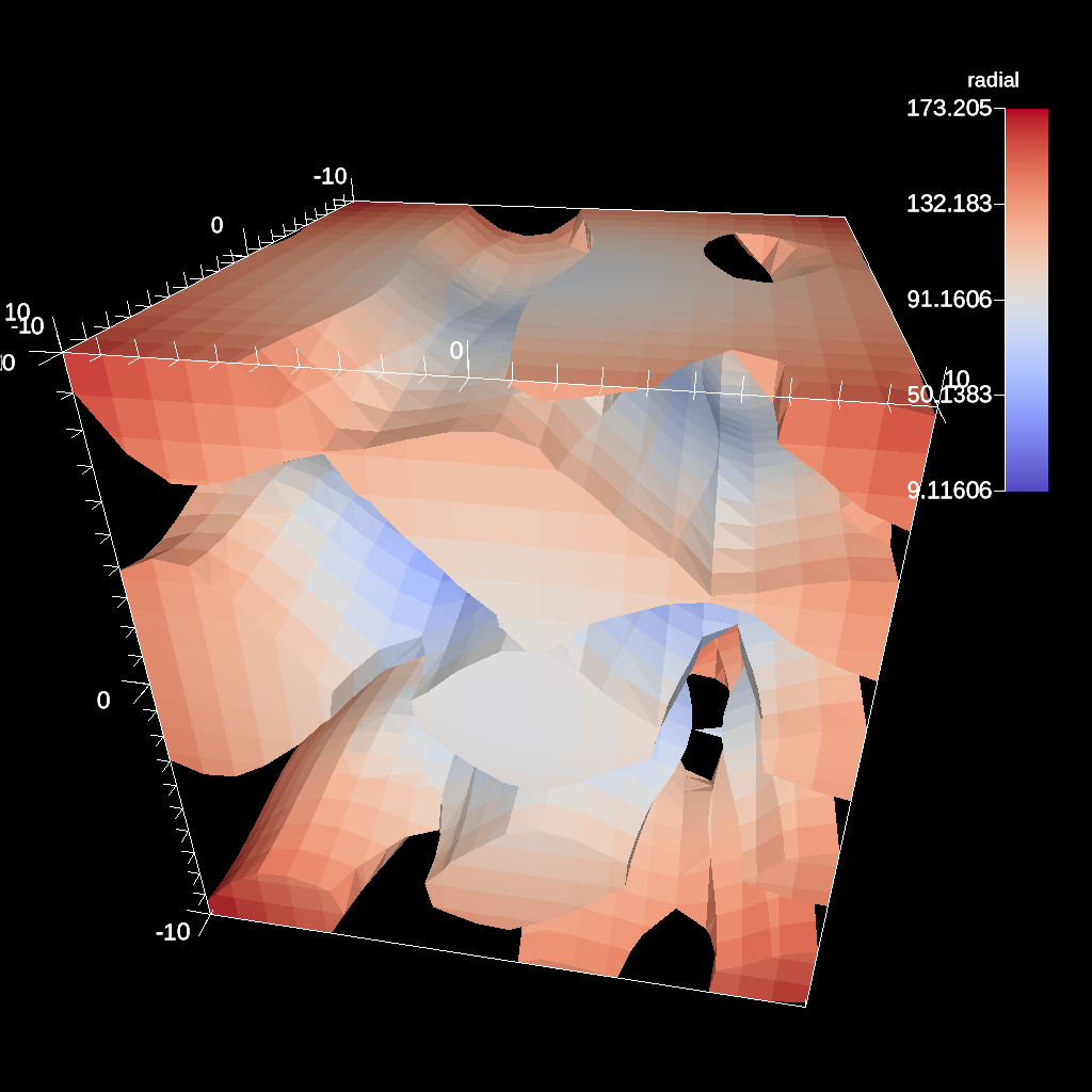
Fig. 39 An example of clipping all values below 0 in a data set.

conduit::Node pipelines;
// pipeline 1
pipelines["pl1/f1/type"] = "clip_with_field";
// filter knobs
conduit::Node &clip_params = pipelines["pl1/f1/params"];
clip_params["field"] = "braid";
clip_params["invert"] = "true";
clip_params["clip_value"] = 0.;

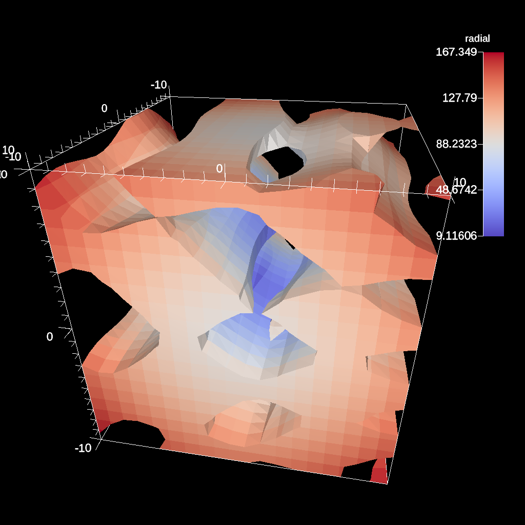
Fig. 40 An example of clipping all values above 0 in a data set.

IsoVolume

IsoVolume is a filter that clips a data set based on a minimum and maximum value in a scalar field. All value outside of the minimum and maximum values are removed from the data set.

conduit::Node pipelines;
// pipeline 1
pipelines["pl1/f1/type"] = "iso_volume";
// filter knobs
conduit::Node &clip_params = pipelines["pl1/f1/params"];
clip_params["field"] = "braid";
clip_params["min_value"] = 5.;
clip_params["max_value"] = 10.;

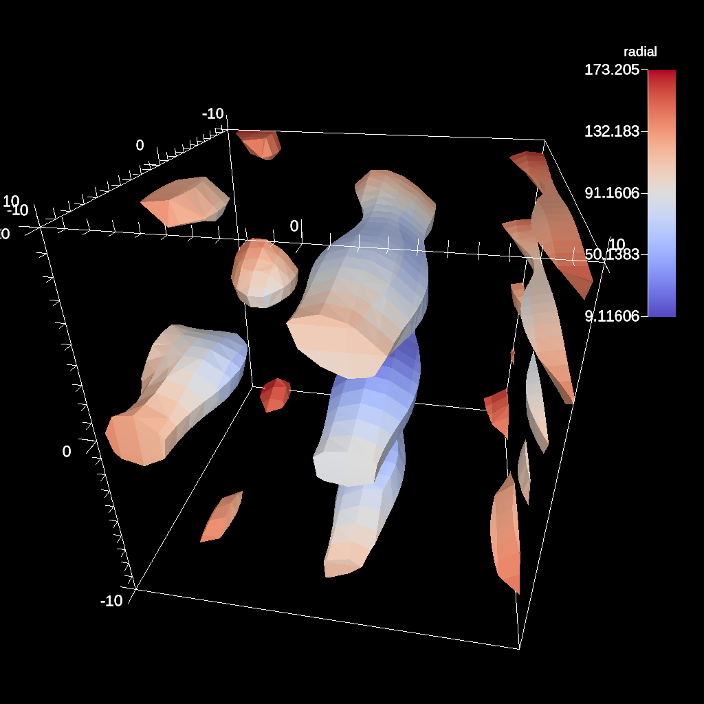
Fig. 41 An example of creating a iso-volume of values between 5.0 and 10.0.

Vector Magnitude

Vector magnitude creates a new field on the data set representing the magitude of a vector variable. The only parameters are the input vector field name and the name of the new field.

conduit::Node pipelines;
// pipeline 1
pipelines["pl1/f1/type"] = "vector_magnitude";
// filter knobs (all these are optional)
conduit::Node &params = pipelines["pl1/f1/params"];
params["field"] = "vel";         // name of the vector field
params["output_name"] = "mag";   // name of the output field

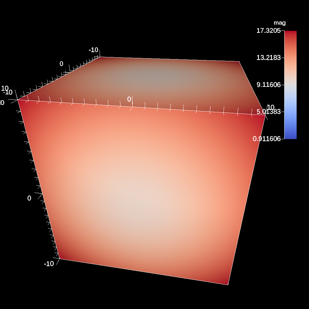
Fig. 42 An example of creating a pseudocolor plot of vector magnitude

Vector Component

Vector component creates a new scalar field on the data set by extracting a component of a vector field. There are three required parameters: the input field, the output field name, and the index of the component to extract.

conduit::Node pipelines;
// pipeline 1
pipelines["pl1/f1/type"] = "vector_component";
// filter knobs (all these are optional)
conduit::Node &params = pipelines["pl1/f1/params"];
params["field"] = "vel";         // name of the vector field
params["output_name"] = "vel_x"; // name of the output field
params["component"] = 0; // index of the component

Composite Vector

Composite Vector creates a new vector field on the data set by combining two or three scalar fields into a vector. The first two fields are required and the presense of the third field dictates whether a 2D or 3D vector is created. Input fields can be different types (e.g., int32 and float32), and the resulting vector field will be a float64.

conduit::Node pipelines;
// pipeline 1
pipelines["pl1/f1/type"] = "composite_vector";
// filter knobs (all these are optional)
conduit::Node &params = pipelines["pl1/f1/params"];
params["field1"] = "pressure";      // (required)
params["field2"] = "temperature";   // (required)
params["field3"] = "bananas";       // (optional, 2D vector if not present)
params["output_name"] = "my_vec";   // (required) name of the output field
params["component"] = 0; // (required) index of the component

Recenter

Recenter changes the association of a field. Fields associated with either element or vertex can be interchanged by averaging the surrounding values. When recentering to a element associated field, all vertex values incident to a element are averaged, and similarly when rencentering to a vertex associated field, all element values incident to the vertex are averaged. If a field is already of the desired associated, then the nothing is done and the field is simply passed through the filter. Note: ghost zones must be available when the data set has more than one domain. Without ghost, the averaging will not be smooth across domain boundaries.

conduit::Node pipelines;
// pipeline 1
pipelines["pl1/f1/type"] = "recenter";
conduit::Node &params = pipelines["pl1/f1/params"];
params["field"] = "braid";         // name of the vector field
params["association"] = "vertex";   // output field association
// or params["association"] = "element";   // output field association

Gradient

Computes the gradient of a vertex-centered input field for every element in the input data set. Fields will be automaticall recentered if they are elemenet-centered. The gradient computation can either generate cell center based gradients, which are fast but less accurate, or more accurate but slower point based gradients (default).

conduit::Node pipelines;
// pipeline 1
pipelines["pl1/f1/type"] = "gradient";
// filter knobs (all these are optional)
conduit::Node &params = pipelines["pl1/f1/params"];
params["field"] = "velocity";          // (required)
params["output_name"] = "my_grad";     // (required) name of the output field
params["use_cell_gradient"] = "false"; // (optional)

Vorticity

Computes the vorticity of a vertex-centered input field for every element in the input data set. Fields will be automaticall recentered if they are elemenet-centered. The vorticity computation (based on the gradient) can either generate cell center based gradients, which are fast but less accurate, or more accurate but slower point based gradients (default).

conduit::Node pipelines;
// pipeline 1
pipelines["pl1/f1/type"] = "vorticity";
// filter knobs (all these are optional)
conduit::Node &params = pipelines["pl1/f1/params"];
params["field"] = "velocity";          // (required)
params["output_name"] = "my_vorticity";// (required) name of the output field
params["use_cell_gradient"] = "false"; // (optional)

Q-Criterion

Computes the qcriterion of a vertex-centered input field for every element in the input data set. Fields will be automaticall recentered if they are elemenet-centered. The qcriterion computation (based on the gradient) can either generate cell center based gradients, which are fast but less accurate, or more accurate but slower point based gradients (default).

conduit::Node pipelines;
// pipeline 1
pipelines["pl1/f1/type"] = "qcriterion";
// filter knobs (all these are optional)
conduit::Node &params = pipelines["pl1/f1/params"];
params["field"] = "velocity";          // (required)
params["output_name"] = "my_q";        // (required) name of the output field
params["use_cell_gradient"] = "false"; // (optional)

Partitioning

Partitioning meshes is commonly needed in order to evenly distribute work among many simulation ranks. Ascent utilizes the partition() functions provided from Conduit::Blueprint. Blueprint provides two partition() functions that can be used to split or recombine Blueprint meshes in serial or parallel. Full M:N repartioning is supported. The partition() functions are in the serial and parallel Blueprint libraries, respectively.

// Serial
void conduit::blueprint::mesh::partition(const Node &mesh,
                                         const Node &options,
                                         Node &output);

// Parallel
void conduit::blueprint::mpi::mesh::partition(const Node &mesh,
                                              const Node &options,
                                              Node &output,
                                              MPI_Comm comm);

Partitioning meshes using Blueprint will use any options present to determine how the partitioning process will behave. Typically, a caller would pass options containing selections if pieces of domains are desired. The partitioner processes any selections and then examines the desired target number of domains and will then decide whether domains must be moved among ranks (only in parallel version) and then locally combined to achieve the target number of domains. The combining process will attempt to preserve the input topology type for the output topology. However, in cases where lower topologies cannot be used, the algorithm will promote the extracted domain parts towards more general topologies and use the one most appropriate to contain the inputs.

In parallel, the partition() function will make an effort to redistribute data across MPI ranks to attempt to balance how data are assigned. Domains produced from selections are assigned round-robin across ranks from rank 0 through rank N-1 until all domains have been assigned. This assignment is carried out after extracting selections locally so they can be restributed among ranks before being combined into the target number of domains.

Fig. 43 Partition used to re-partition a 7 domain mesh (left) to different target numbers of domains and to isolate logical subsets.

Options

The partition() functions accept a node containing options. The options node can be empty and all options are optional. If no options are given, each input mesh domain will be fully selected. It is more useful to pass selections as part of the option node with additional options that tell the algorithm how to split or combine the inputs. If no selections are present in the options node then the partitioner will create selections of an appropriate type that selects all elements in each input domain.

The target option is useful for setting the target number of domains in the final output mesh. If the target value is larger than the number of input domains or selections then the mesh will be split to achieve that target number of domains. This may require further subdividing selections. Alternatively, if the target is smaller than the number of selections then the selections will be combined to yield the target number of domains. The combining is done such that smaller element count domains are combined first. Additionally, Ascent provides an optional boolean parameter, distributed, which dictates if the number of chosen target domains is applied across ranks (true, default), or to each rank individually (false).

Option	Description	Example
selections	A list of selection objects that identify regions of interest from the input domains. Selections can be different on each MPI rank.	selections: - type: logical start: [0,0,0] end: [9,9,9] domain_id: 10
target	An optional integer that determines the fields containing original domains and number of domains in the output. If given, the value must be greater than 0. Values larger than the number of selections cause domains to be split. Values smaller than the number of selections cause domains to be combined. Invalid values are ignored. If not given, the output will contain the number of selections. In parallel, the largest target value from the ranks will be used for all ranks.	target: 4
fields	An list of strings that indicate the names of the fields to extract in the output. If this option is not provided, all fields will be extracted.	fields: ["dist", "pressure"]
mapping	An integer that determines whether fields containing original domains and ids will be added in the output. These fields enable one to know where each vertex and element came from originally. Mapping is on by default. A non-zero value turns it on and a zero value turns it off.	mapping: 0
merge_tolerance	A double value that indicates the max allowable distance between 2 points before they are considered to be separate. 2 points spaced smaller than this distance will be merged when explicit coordsets are combined.	merge_tolerance: 0.000001
distributed	An optional boolean value for parallel execution. If true, the chosen number of target domains will be applied across all ranks. If false, the chosen number of target domains will be applied to each rank individually. If not given, the default is true.	distributed: "false"

Selections

Selections can be specified in the options for the partition() function to select regions of interest that will participate in mesh partitioning. If selections are not used then all elements from the input meshes will be selected to partitipate in the partitioning process. Selections can be further subdivided if needed to arrive at the target number of domains. Selections can target specific domains and topologies as well. If a selection does not apply to the input mesh domains then no geometry is produced in the output for that selection.

The partition() function’s options support 4 types of selections:

Selection Type	Topologies	Description
logical	uniform,rectilinear,structured	Identifies start and end logical IJK ranges to select sub-bricks of uniform, rectilinear, or structured topologies. This selection is not compatible with other topologies.
explicit	all	Identifies an explicit list of element ids and it works with all topologies.
ranges	all	Identifies ranges of element ids, provided as pairs so the user can select multiple contiguous blocks of elements. This selection works with all topologies
field	all	Uses a specified field to indicate destination domain for each element.

By default, a selection does not apply to any specific domain_id. A list of selections applied to a single input mesh will extract multiple new domains from that original input mesh. Since meshes are composed of many domains in practice, selections can also be associated with certain domain_id values. Selections that provide a domain_id value will only match domains that either have a matching state/domain_id value or match its index in the input node’s list of children (if state/domain_id is not present).

Selections can apply to certain topology names as well. By default, the first topology is used but if the topology name is provided then the selection will operate on the specified topology only.

Option	Description	Example
type	The selection type	selections: - type: logical
domain_id	The domain_id to which the selection will apply. This is almost always an unsigned integer value. For field selections, domain_id is allowed to be a string “any” so a single selection can apply to many domains.	selections: - type: logical domain_id: 10 selections: - type: logical domain_id: any
topology	The topology to which the selection will apply.	selections: - type: logical domain_id: 10 topology: mesh

Logical Selection

The logical selection allows the partitioner to extract a logical IJK subset from uniform, rectilinear, or structured topologies. The selection is given as IJK start and end values. If the end values extend beyond the actual mesh’s logical extents, they will be clipped. The partitioner may automatically subdivide logical selections into smaller logical selections, if needed, preserving the logical structure of the input topology into the output.

selections:
  -
   type: logical
   start: [0,0,0]
   end: [9,9,9]

Explicit Selection

The explicit selection allows the partitioner to extract a list of elements. This is used when the user wants to target a specific set of elements. The output will result in an explicit topology.

selections:
  -
   type: explicit
   elements: [0,1,2,3,100,101,102]

Ranges Selection

The ranges selection is similar to the explicit selection except that it identifies ranges of elements using pairs of numbers. The list of ranges must be a multiple of 2 in length. The output will result in an explicit topology.

selections:
  -
   type: ranges
   ranges: [0,3,100,102]

Field Selection

The field selection enables the partitioner to use partitions done by other tools using a field on the mesh as the source of the final domain number for each element. The field must be associated with the mesh elements. When using a field selection, the partitioner will make a best attempt to use the domain numbers to extract mesh pieces and reassemble them into domains with those numberings. If a larger target value is specified, then field selections can sometimes be partitioned further as explicit partitions. The field selection is unique in that its domain_id value can be set to “any” if it is desired that the field selection will be applied to all domains in the input mesh. The domain_id value can still be set to specific integer values to limit the set of domains over which the selection will be applied.

selections:
  -
   type: field
   domain_id: any
   field: fieldname