Scenes

A scene encapsulates the information required to generate one or more images. To define a scene, the user specifies a collection of plots (e.g., volume or surface rendering) and associated parameters such as camera definitions, light positions, and annotations. The simplest plot description requires only a plot type and scalar field name. A scene defined in this way uses the default data source, which is all of the data published by the simulation, and default settings for camera position, image resolution, lighting, and annotations.

Default Images

When creating a scene, Ascent will set up camera and color table defualts. The only requirement is that either a image_name or image_prefix be provided. Minimally, a scene consists of one plot and a parameter to specify the output file name. Default images images have a resolution of 1024x1024.

conduit::Node scenes;
scenes["s1/plots/p1/type"]  = "pseudocolor";
scenes["s1/plots/p1/field"] = "braid";
// scene default image prefix
scenes["s1/image_prefix"] = output_file_name;

If anything other than the default camera, annotation, image resolution, or color table parameters are needed, then a render will need to be specified. Renders are covered later in this section.

Image Prefix

The image_prefix is a string denotes a prefix to be used when saving the image. For multiple cycles, the cycle number will be appended to the image filename. Numeric formatting, similar to printf is supported within the image prefix. Assuming the cycle is 10, here are some examples:

• image_: image_10.png

• image_%04d: image_0010.png

Image Name

The image_name parameter speficies the excact file name of the of the output image, and Ascent will append the .png to the image file name. If not changed, the image file will be overwritten.

Plots

We current have support for three plot types: pseudocolor, volume, and mesh. Both plots support node centered and element centered scalar fields. Plots optionally consume the result of a pipeline, but if none is specified, then the plot input is the published mesh data. Each scene can contain one or more plots. The plot interface is simply:

{
  "type"   : "plot_name",
  "pipeline" : "pipeline_name",
  "field" : "field_name"
}

In c++, the equivalent declarations would be as follows:

conduit::Node plot;
plot["type"] = "plot_name";
plot["pipeline"] = "pipeline_name";
plot["field"] = "field_name";

Pseudocolor

A pseudocolor plot simply renders the mesh coloring by the provided scalar field. Below is an example of creating a scene with a single pseudocolor plot with the default pipeline:

conduit::Node scenes;
scenes["s1/plots/p1/type"]         = "pseudocolor";
scenes["s1/plots/p1/field"] = "braid";
// scene default image prefix
scenes["s1/image_prefix"] = output_file_name;

conduit::Node actions;
conduit::Node &add_plots = actions.append();
add_plots["action"] = "add_scenes";
add_plots["scenes"] = scenes;

An example of creating a scene with a user defined pipeline:

conduit::Node pipelines;
// pipeline 1
pipelines["pl1/f1/type"] = "contour";
// filter knobs
conduit::Node &contour_params = pipelines["pl1/f1/params"];
contour_params["field"] = "braid";
contour_params["iso_values"] = 0.;

conduit::Node scenes;
scenes["s1/plots/p1/type"]         = "pseudocolor";
scenes["s1/plots/p1/field"] = "radial";
scenes["s1/plots/p1/pipeline"] = "pl1";
scenes["s1/image_prefix"] = output_file;

conduit::Node actions;
// add the pipeline
conduit::Node &add_pipelines= actions.append();
add_pipelines["action"] = "add_pipelines";
add_pipelines["pipelines"] = pipelines;
// add the scenes
conduit::Node &add_scenes= actions.append();
add_scenes["action"] = "add_scenes";
add_scenes["scenes"] = scenes;

In addition to surfaces, this pseudocolor color plot can render point meshes with no additional parameters. While there is a default point radius, the plot options allow for constant or variable radii.

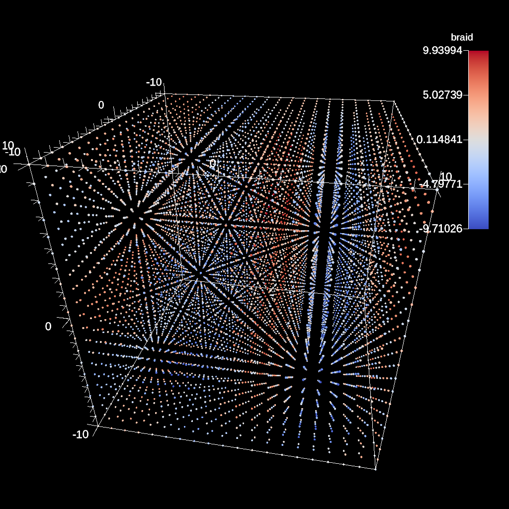
Fig. 44 Default heuristic for points size

conduit::Node scenes;
scenes["s1/plots/p1/type"]         = "pseudocolor";
scenes["s1/plots/p1/field"] = "braid";
scenes["s1/plots/p1/points/radius"] = 1.f;

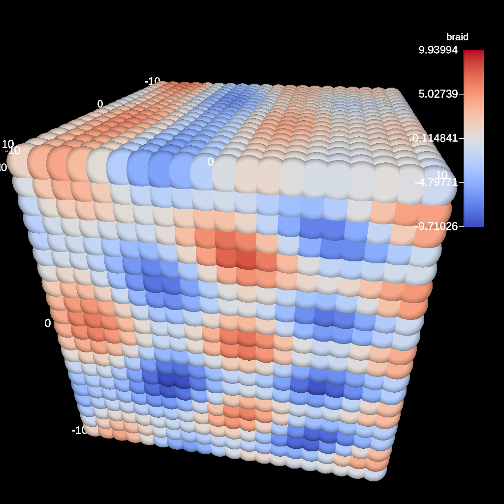
Fig. 45 Point mesh rendered with a constant radius

For variable radii, the field values are used to scale each points radius relative to the global min and max scalar value. The inputs are the base radius size, and the delta (multiplier) of the radius. In the example below, scalar values at the minimum of the scalar range will have a radius of 0.25 and scalar values at the max will have radii of 0.25 + 0.5.

conduit::Node scenes;
scenes["s1/plots/p1/type"]  = "pseudocolor";
scenes["s1/plots/p1/field"] = "braid";
scenes["s1/plots/p1/points/radius"] = 0.25f;
// this detla is relative to the base radius
scenes["s1/plots/p1/points/radius_delta"] = 2.0f;

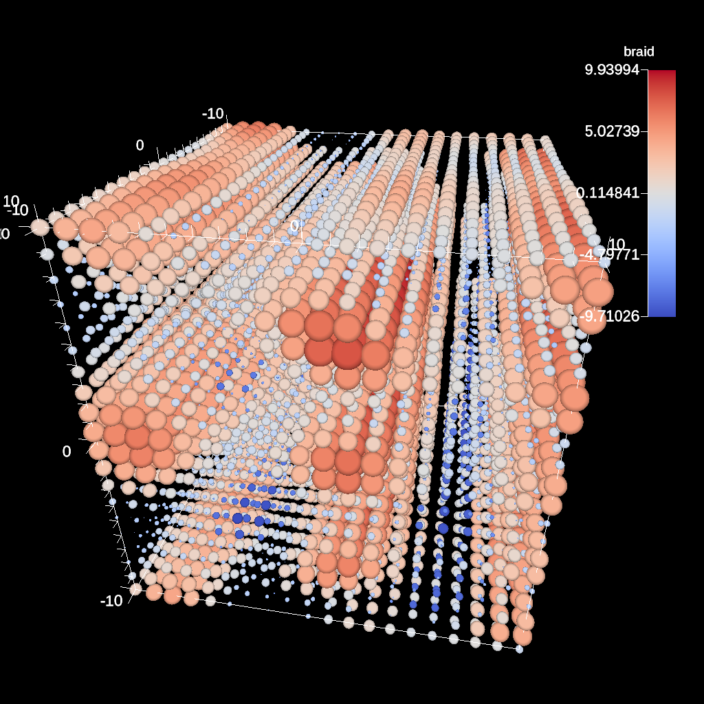
Fig. 46 Point mesh rendered with a variable radius

Volume Plot

The volume plot produces a volume rendering of the provided scalar field. The code below creates a volume plot of the default pipeline.

conduit::Node scenes;
scenes["s1/plots/p1/type"]  = "volume";
scenes["s1/plots/p1/field"] = "braid";

conduit::Node actions;
conduit::Node &add_plots = actions.append();
add_plots["action"] = "add_scenes";
add_plots["scenes"] = scenes;

Mesh Plot

The mesh plot, displays the computational mesh over which the simulations variables are defined. The mesh plot is often added to the scene window when other plots are visualized to allow individual cells to be clearly seen. The code below creates a volume plot of the default pipeline.

conduit::Node scenes;
scenes["s1/plots/p1/type"]  = "mesh";

conduit::Node actions;
conduit::Node &add_plots = actions.append();
add_plots["action"] = "add_scenes";
add_plots["scenes"] = scenes;

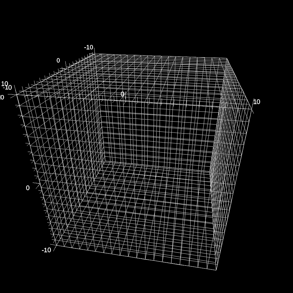
Fig. 47 A mesh plot of simple grid.

Color Tables

The color map translates normalized scalars to color values. Color maps can be applied to each each plot in a scene. Image of the color tables provided by VTK-m can be found in VTK-m Color Tables. Minimally, a color table name needs to be specified, but the color_table node allows you to specify RGB and Alpha (opacity) control points for complete customization of color maps. Alpha control points are used when rendering volumes. The built-in Color map names are: Cool to Warm, Black-Body Radiation, Samsel Fire, Inferno, Linear YGB, Cold and Hot, Rainbow Desaturated, Cool to Warm (Extended), X Ray, Black, Blue and White, Viridis, Linear Green, Jet, and Rainbow. Colors are three double precision values between 0 and 1. Alphas and positions are a single double precision values between 0 and 1.

Here is an example of specifying a color table by name:

conduit::Node scenes;
scenes["s1/plots/p1/type"]  = "pseudocolor";
scenes["s1/plots/p1/field"] = "braid";
scenes["s1/plots/p1/color_table/name"] = "Viridis";

Color in the table can be reversed through an optional parameter:

scenes["s1/plots/p1/color_table/reverse"] = "true";

Volume plots are special since ray casting blends colors together. When no color table is specified, alpha values are automatically created, but when a color table is specified, then the color table needs to include alpha values. Otherwise, the volume plot will look exactly the same as a pseudocolor plot.

Here is an example of adding a custom color table to the volume plot:

conduit::Node control_points;
conduit::Node &point1 = control_points.append();
point1["type"] = "rgb";
point1["position"] = 0.;
double color[3] = {1., 0., 0.};
point1["color"].set_float64_ptr(color, 3);

conduit::Node &point2 = control_points.append();
point2["type"] = "rgb";
point2["position"] = 0.5;
color[0] = 0;
color[1] = 1.;
point2["color"].set_float64_ptr(color, 3);

conduit::Node &point3 = control_points.append();
point3["type"] = "rgb";
point3["position"] = 1.0;
color[1] = 0;
color[2] = 1.;
point3["color"].set_float64_ptr(color, 3);

conduit::Node &point4 = control_points.append();
point4["type"] = "alpha";
point4["position"] = 0.;
point4["alpha"] = 0.;

conduit::Node &point5 = control_points.append();
point5["type"] = "alpha";
point5["position"] = 1.0;
point5["alpha"] = 1.;

conduit::Node scenes;
scenes["s1/plots/p1/type"]  = "volume";
scenes["s1/plots/p1/field"] = "braid";
scenes["s1/plots/p1/color_table/control_points"] = control_points;

conduit::Node actions;
conduit::Node &add_plots = actions.append();
add_plots["action"] = "add_scenes";
add_plots["scenes"] = scenes;

Clamping Scalar Values

The minimum and maximum values of a scalar field varies with each simulation time step, and rendering plots of the same field from different time steps causes inconsistent mappings from scalars values to colors. To create a consistent mapping, a plot has two optional parameters that clamp the scalar values to a given range. Any scalar value above the maximum value will be clamped to the maximum, and any scalar value below the minimum value will be clamped to the minimum.

Here is an example of clamping the scalar values to the range [-0.5, 0.5].

conduit::Node scenes;
scenes["s1/plots/p1/type"]  = "pseudocolor";
scenes["s1/plots/p1/field"] = "braid";
scenes["s1/plots/p1/min_value"] = -0.5;
scenes["s1/plots/p1/max_value"] = 0.5;

Renders (Optional)

Scenes contains a list of Renders that specify the parameters of a single image. If no render is specified, a default render is created automatically. Here is an example of creating a scene with render with some basic parameters:

conduit::Node scenes;
scenes["s1/plots/p1/type"]  = "pseudocolor";
scenes["s1/plots/p1/field"] = "braid";
scenes["s1/image_prefix"] = output_file;

scenes["s1/renders/r1/image_width"]  = 512;
scenes["s1/renders/r1/image_height"] = 512;
scenes["s1/renders/r1/image_name"]   = output_file;

Now we add a second render to the same example using every available parameter:

scenes["s1/renders/r2/image_width"]  = 300;
scenes["s1/renders/r2/image_height"] = 400;
scenes["s1/renders/r2/image_name"]   = output_file2;
double vec3[3];
vec3[0] = 1.; vec3[1] = 1.; vec3[2] = 1.;
scenes["s1/renders/r2/camera/look_at"].set_float64_ptr(vec3,3);
vec3[0] = 15.; vec3[1] = 17.; vec3[2] = 15.;
scenes["s1/renders/r2/camera/position"].set_float64_ptr(vec3,3);
vec3[0] = 0.; vec3[1] = -1.; vec3[2] = 0.;
scenes["s1/renders/r2/camera/up"].set_float64_ptr(vec3,3);
scenes["s1/renders/r2/camera/fov"] = 45.;
scenes["s1/renders/r2/camera/xpan"] = 1.;
scenes["s1/renders/r2/camera/ypan"] = 1.;
scenes["s1/renders/r2/camera/azimuth"] = 10.0;
scenes["s1/renders/r2/camera/elevation"] = -10.0;
scenes["s1/renders/r2/camera/zoom"] = 3.2;
scenes["s1/renders/r2/camera/near_plane"] = 0.1;
scenes["s1/renders/r2/camera/far_plane"] = 33.1;

{
"renders":
{
  "r1":
  {
    "image_width": 300,
    "image_height": 400,
    "image_name": "some_image",
    "camera":
    {
      "look_at": [1.0, 1.0, 1.0],
      "position": [0.0, 25.0, 15.0],
      "up": [0.0, -1.0, 0.0],
      "fov": 60.0,
      "xpan": 0.0,
      "ypan": 0.0,
      "elevation": 10.0,
      "azimuth": -10.0,
      "zoom": 0.0,
      "near_plane": 0.1,
      "far_plane": 100.1
    }
  }
}
}

Additional Render Options

In addition to image and camera parameters, renders have several options that allow the users to control the appearance of images. Below is a list of additional parameters:

• bg_color : an array of three floating point values that controls the background color.

• fg_color : an array of three floating point values that controls the foreground color. The foreground color is used to color annotations and mesh plot lines.

• annotations : controls if annotations are rendered or not. Valid values are "true" and "false".

• render_bg : controls if the background is rendered or not. If no background is rendered, the background will appear transparent. Valid values are "true" and "false".

• dataset_bounds : controls the dimensions of the rendered bounding box around the dataset. This will overwrite the default bounding box based on the dataset’s dimensions. A valid value is an array of six floats ([xMin,xMax,yMin,yMax,zMin,zMax]) that define dimensions larger than the default. Note: this does not control annotations. To turn off dataset annotations, see An example of rendering with no world annotations.. To turn off screen annotations, see An example of rendering with no screen annotations..

• color_bar_position : controls the position of 1 or more color bars. A valid value for positioning a single color bar is an array of four floats ([xMin,xMax,yMin,yMax]). A valid value for positioning N color bars is an array of 4*N floats ([xMin1_0,xMax1_0,yMin1_0,yMax1_0,…,xMin_n,xMax_n,yMin_n,yMax_n]). This repositioning is performed in Screen Space, so valid minimum and maximum values are limited to the range [-1,1] (i.e. the origin (0,0) is in the center of the image, (-1,-1) is the bottom-left corner, and (1,1) is the top-right corner). Note: Ascent does not check for correctness of user positioned color bars.

Automatic Camera

The automatic camera render is used to automatically choose a camera placement, basing the decision on a user-chosen viewpoint quality (VQ) metric. The automatic camera render requires a mesh and scalar field data, and works in conjunction with other Filters. The automatic camera render analyzes the data that will be rendered using a user-chosen metric and number of considered cameras. Given the number of cameras, the camera placements are determined using Fibonacci’s Lattice, a method for placing points around a unit sphere, and the camera is pointed at the center of the data.

A user can specify the number of camera samples (auto_camera/samples) to consider when determining the best camera placement. The user also specifies the field data (auto_camera/field) the VQ metric will operate on, as well as the VQ metric (auto_camera/metric). The current VQ metrics and respective keywords are:

Data Entropy : data_entropy Depth Entropy : depth_entropy Shading Entropy : shading_entropy DDS Entropy : dds_entropy

There are also several optional parameters a user can specify, such as the number of bins (auto_camera/bins=256) to be used in the entropy calculations, as well as height (auto_camera/height=1024) and width (auto_camera/width=1024).

Usage Recommendation: Automatically producing quality camera placements is a difficult task, and not all of the available VQ metrics consistently produce viewpoints that users want to see or find insightful. If users do not have a prior preference, we recommend using the VQ metric DDS Entropy, which is the sum of Data Entropy, Depth Entropy, and Shading Entropy. Marsaglia et al. cite{marsaglialdav} performed a user study that showed that out of the available VQ metrics, DDS Entropy produces viewpoints that scientific experts prefer.

The code below creates a pipeline that first applies a contour filter and then applies the camera filter before declaring a scene.

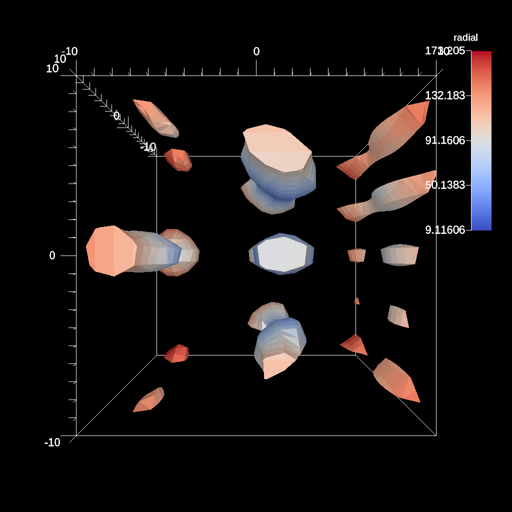
Fig. 48 The default camera placement for this example.

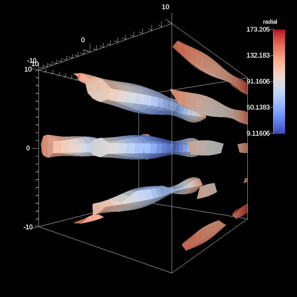
Fig. 49 The camera placement chosen by the VQ metric DDS Entropy for this example. This example and implementation of the other VQ metrics can be found in auto_camera test.

Cinema Databases

The Cinema specification is a image-based solution for post-hoc exploration of simulation data. The idea behind Cinema is images take many orders of magnitude less disk space than that of the entire simulation data. By saving images instead of the full mesh, we can save data much more frequently, giving users access to more temporal fidelity than would be possible otherwise. For a complete overview, see the SC 14 paper. Other Cinema resources can be found at Cinema Science.

Ascent currently supports the creation of the Astaire specification (spec A) which captures images of the scene from positions on a spherical camera. The number of images are captured in the parameters phi and theta. phi specifies the number of divisions along the polar angle and theta specifies the number of divisions along the azimuth. For example, if phi = 4 and theta = 8 then the resulting database will contain 4 * 8 images per time step. The Cinema database can then be explored in a supported viewer. In the future we hope to integrate a web-based viewer to enable exploration of the Cinema database as the simulation is running.

conduit::Node scenes;
scenes["scene1/plots/plt1/type"]         = "pseudocolor";
scenes["scene1/plots/plt1/params/field"] = "braid";
// setup required cinema params
scenes["scene1/renders/r1/type"] = "cinema";
scenes["scene1/renders/r1/phi"] = 2;
scenes["scene1/renders/r1/theta"] = 2;
scenes["scene1/renders/r1/db_name"] = "example_db";

A full code example can be found in the test suite’s Cinema test.