Data Binning
Ascent’s Data Binning was modeled after VisIt’s Data Binning / Derived Data Field capability. The capability defies a good name, it is has also been called Equivalence Class Functions. The approach is very similar to a multi-dimensional histogram. You define a multi-dimensional binning, based on either spatial coordinates or field values, and then Ascent will loop over your mesh elements and aggregate them into these bins. During the binning process, you can employ a menu of reduction functions (sum, average, min, max, variance, etc) depending on the type of analysis desired.
You can bin spatially to calculate distributions, find extreme values, etc. With the right approach, you can implement mesh agnostic analysis that can be used across simulation codes. You can also map the binned result back onto the original mesh topology to enable further analysis, like deviations from an average.
Benefits
Simulation user often needs to analyze quantities of interest within fields on a mesh, but the user might not know the exact data structures used by the underlying simulation. For example, the mesh data might be represented as uniform grids or as high-order finite element meshes. If the users does not know the underlying data structures, it can be very difficult to write the underlying analysis, and that analysis code will not work for another simulation. Using spatial binning essentially create a uniform representation that can be use across simulation codes, regardless of the underlying mesh representation.
Sampling and Aggregation
When specifying the number of bins on an axis, there will always be over sampling or undersampling. During spatial binning, each zone is placed into a bin based on its centroid, and as with all binning, this is subject to over sampling or under sampling.
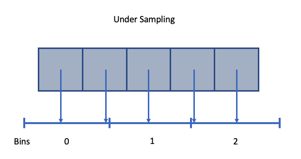
Fig. 56 An example of spatial under sampling.
When multiple values fall into a single bin (i.e., undersampling), we aggregate values using the following options:
min: minimum value in a bin
max: maximum value in a bin
sum: sum of values in a bin
avg: average of values in a bin
pdf: probability distribution function
std: standard deviation of values in a bin
var: variance of values in a bin
rms: root mean square of values in a bin
The aggregation function is the second argument to the binning function and is demonstrated in the line out example.
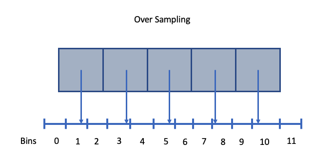
Fig. 57 An example of spatial over sampling.
When oversampling data, the default value of an empty bin is 0. That said, the default empty value can be overridden by an option named parameter, e.g., empty_bin_val=100. This is often useful when the default value is part of the data range, and setting the empty bin value to something known, allows the user to filter out empty bins from the results.
Example Line Out
We will use data binning to provide capability similar to a a line out. To accomplish this, we will define a spatial binning that is like a pencil down the center of the data set in the z direction, and we will use the noise mini-app to demonstrate.
In the Lulesh proxy application, the mesh is defined with the spatial bounds (0,0,0)-(1.2,1.2,1.2). We will define a three dimensional binning on the ranges x=(0,0.1) with 1 bin, y=(0,1.2) with 1 bin, and z=(0,1.2) with 20 bins. This is technically a 3d binning, but it will result in a 1d array of values.
Lusesh implements the Sedov blast problem which deposits a region of high energy in one corner of the data set, and as time progresses, a shockwave propagate out. The idea behind this example is to create a simple query to help us track the shock front as it moves through the problem. To that end, we will create a query that bins pressure (i.e., the variable p).
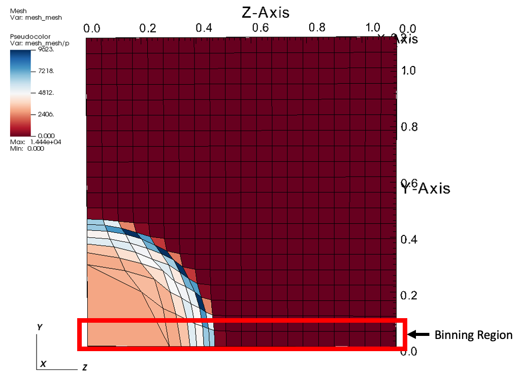
Fig. 58 An example of Lulesh where the binning region is highlighted in red..
Actions File
An example ascent actions file that create this query:
-
  action: "add_queries"
  queries:
    bin_density:
      params:
        expression: "binning('p','max', [axis('x',[0.0,0.1]), axis('y', [0.0,0.1]), axis('z', num_bins=20)])"
        name: my_binning_name
Note that with and x and y axes that we are explicitly specifying the bounds of the bins. Ascent deduces the number of bins bases on the explicit coordinates inside the array [0.0,0.1]. With the z axis, the binning automatically defines a uniform binning based on the spatial extents of the mesh. Additionally, we are using max as the aggregation function.
Session File
The binning is called every cycle ascent is executed, and the results are stored within the expressions cache. When the run is complete, the results of the binning, as well as all other expressions, are output inside the ascent_session.yaml file, which is convenient for post processing.
Here is a excerpt from the session file (note: the large array is truncated):
my_binning_name:
  1:
    type: "binning"
    attrs:
      value:
        value: [0.0, ...]
        type: "array"
      reduction_var:
        value: "p"
        type: "string"
      reduction_op:
        value: "max"
        type: "string"
      bin_axes:
        value:
          x:
            bins: [0.0, 0.1]
            clamp: 0
          y:
            bins: [0.0, 0.1]
            clamp: 0
          z:
            num_bins: 20
            clamp: 0
            min_val: 0.0
            max_val: 1.12500001125
      association:
        value: "element"
        type: "string"
    time: 1.06812409221472e-05
Inside the session file is all the information Ascent used to create the binning, including the automatically defined spatial ranges for the z axis, fields used, the aggregate operation, cycle, and simulation time. The session file will include an entry like the one above for each cycle, and the cycle is located directly below the name of the query (i.e., my_binning_name). Once the simulation is complete, we can create a python script to process and plot the data.
Plotting
Plotting the resulting data is straight forward in python.
import yaml #pip install --user pyyaml
import pandas as pd
import matplotlib.pyplot as plt

session = []
with open(r'ascent_session.yaml') as file:
  session = yaml.load(file)

binning = session['binning']
cycles = list(binning.keys())
bins = []

# loop through each cycle and grab the bins
for cycle in binning.values():
  bins.append((cycle['attrs']['value']['value']))

# create the coordinate axis using bin centers
z_axis = binning[cycles[0]]['attrs']['bin_axes']['value']['z']
z_min = z_axis['min_val']
z_max = z_axis['max_val']
z_bins = z_axis['num_bins']

z_delta = (z_max - z_min) / float(z_bins)
z_start = z_min + 0.5 * z_delta
z_vals = []
for b in range(0,z_bins):
  z_vals.append(b * z_delta + z_start)

# plot the curve from the last cycle
plt.plot(z_vals, bins[-1]);
plt.xlabel('z position')
plt.ylabel('pressure')
plt.savefig("binning.png")
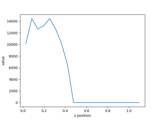
Fig. 59 The resulting plot of pressure from the last cycle.
From the resulting plot, we can clearly see how far the shock front has traveled through the problem. Plotting the curve through time, we can see the shock from move along the z-axis.